Graphing Functions
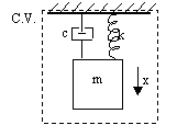
Suppose we wish to graph the behavior of damped oscillations made by a system consisting of a simple (linear) spring and a mass attatched to it from a ceiling. Without entering the small details of the calculation (this is not the purpose of our discussion), here is the solution:
The spring's stiffness is k= 1000 N/m
The mass m is 1 kg
The damping coefficient is c= 10 kg/s
The mass m was given a velocity of 2 m/s in the x positive direction from the point of equilibrium.
And so we would like to see what this function looks like. We will graph it using the TI calculator.
? Why aren't we graphing an "x" function of "t"?
Ans The calculator uses a list of functions, from which it is most convenient to graph. Sort of a "To Do" list of graphs. This list is accessible in the Y= editor, by pressing DIAMOND+F1, for example:
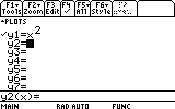
See the list of numbered y's waiting to be graphed? Each y is a function of x, and when it contains an expression of x, and is tagged (with the tick mark) it will be graphed.
To graph our function, we need to name the independent variable x, and not t. Otherwise the calculator will not be able to graph it. It always expects a function of x.
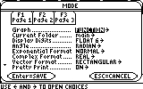
? It doesn't say FUNCTION. What do I do?
Ans If your calculator says otherwise, such as PARAMETRIC or POLAR or any other listing, you will need to change it back to FUNCTION. Use the right arrow while on the Graph line (as indicated above) and choose FUNCTION:
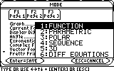
Confirm by pressing ENTER to save your settings.
2. Now that we have "told" our calculator that we wish to graph functions of the form f(x), we can enter our function in the Y= editor.
Open the Y= editor by pressing DIAMOND+F1.
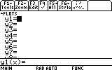
Your Y= editor may show one or more functions already entered. We will need just one of the y#'s free. You can scroll down to a free y# or delete one of the occupied y#'s using the CLEAR button or the Backspace button while the highlight is on the occupied line.
Either way, with the highlight on an empty y# line, we are now ready to enter our function. Start typing and the entry line below will show you what you enter, just like on the home screen. Enter the entire expression:
0.064051*e^(-5x)*sin(31.225x)
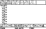
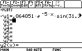
Notice that he newly entered y# is tagged (selected, the manual calls it). If there are any other selected y# in your Y= editor, deselect them by highlighting them and pressing F4. If you leave another y# selected, the calculator will graph it too. They may overlap, take longer to graph, and complicate other actions. We don't want that, do we? Make sure only our expression is selected before we continue.
Next we need to specify the graphing boundaries. It is not easy in this case: we know that we do not need the x<0 range (equivalent to t<0) but we don't know the other boundaries. The simple, straightforward approach of trial and error is the most suitable in this case (why? because the function is small and doesn't take long to evaluate). Let us set the boudaries:
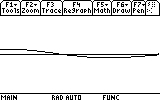
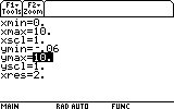
3. Press DIAMOND+F2 for the WINDOW screen. This is where we set the boundaries of the graphed area. Your WINDOW screen setting probably shows different numbers, but as we have learned, this is not an obstacle for us: any setting can be easily changed to suit out needs.
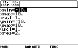
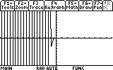
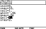
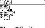
Not very useful is it? Not very physical either: it contains the t<0 range, and that certainly isn't what we need. Next we notice that the interesting part, after t=0 (that is, the t>0 range) is too small in this picture. Obviously the Y range should not be -10..10, but much smaller. Let's go back to the WINDOW settings and change the boundaries. Press DIAMOND+F2 again.
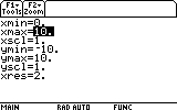
First, change xmin to indicate 0, so that our time axis starts from t=0. We accomplish this by highlighting the xmin= line, typing 0 and pressing ENTER.
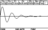
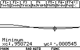
The GRAPH screen is a great place to learn many useful things about our function. For example, where it reaches maximum and minumum values (that is, the amplitude the mass m reaches each time), and when it practically stops oscillating.
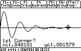
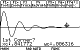
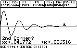
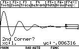
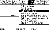
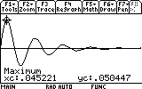
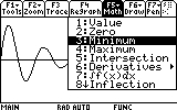
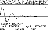
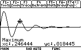
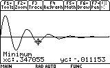
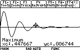
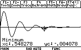
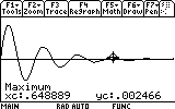
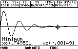
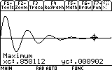
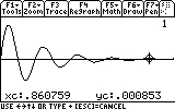
Let's find out how far the mass reaches each oscillation. First the mass reaches the first "peak". Where is that peak located? To see the coordinates of the peak (maximum) we would have to locate it. The graph screen has a tool that does just that. Press F5. Item number 4 says "Maximum".
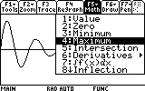

...and press ENTER to comfirm.
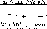
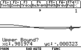
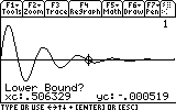
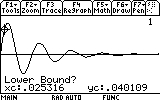
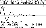
Next we will provide the rightmost point of the search range. Move the cursor somewhat to the right of the minimum...
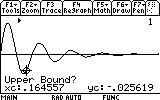
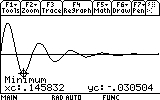
As you can see, the mass now reaches only to 0.03 meters distance from the equilibrium point (instead of 0.05). Repeat the search for the other visible peaks (7 of them... don't be lazy now!). Here are the results:
The last important number that we would like to know is when the oscillations practically stopped. I say practically, because methematically that would me t=infinity. But in reality, all we need to know is when the oscillations become very, very small. As it happens to be, this information is also visible on the GRAPH screen. See how the oscillation virtually "disapear" after the ninth peak? But we should not be satisfied with mere eye sight. Let's actually look into the values the function has after the ninth peak:
To track (or trace) the values of a function, the calculator has a command called, surprise-surprise, Trace, which is activated with F3. Press F3 now.
? Why are the steps such irrational numbers? Why not something a little more logical like 0.01?
Ans The calculator graphs the function using points. The intervals between the points are calculated according to the boundaries of the graph area, the "xres" variable (which means the number of pixels to use for intervals)... In short, you cannot "walk" on a point that's not there.
If we insisted on exactly 0.01 inetrvals, for example, we could have acheived this by manually assigning the deltax variable a value of, say, 0.01, after setting the graph area boundaries. But this is rarely necessary and will not be further discussed here.
Back to our search of the time when the mass stops oscillating -- we must determine a rule of thumb since there is no absolute way of determining this. Let's say that for us the mass stops oscillating when the amplitudes (the peaks) reach 1% or less of the first one. If we look at the last (ninth) peak we checked, there was an amplitude of 0.000902, which is 0.01788 or 1.788% of the first amplitude. That's not enough. Let's look for the next peak. But we cannot even see it! How do we find it? Well, it's time to zoom in!
The zoom option is, again very surprisingly, within the ZOOM (F2) menu. Press F2 now.
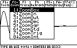
The easiest way to zoom in exactly on the area that interests us is to use zoom box. This way, we could choose a "frame" within which to view the function.
Choose 2:ZoomBox.