Half-Step Root Finding Method
As another example application for the TI-89 or 92+, we will now demonstrate the creation of a simple root finding method. The purpose of this example is to demonstrate programming, plotting, lists and a few other things the TIs can do.
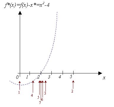
There are several useful features of this method.
- Simple concept, simple application
- Can be applied to almost any procedure which outputs a number and ultimately produces a smooth function†
- Requires a number of iterations which is almost the same for very different ranges‡
- Follows a simple rule when more than one solution exists: If the range contains two of more solutions, the complimentary range will always converge to the other solutions, and never back to the one already found§
† In other words, the expression given to the algorithm can be a complete
procedure in its own right, such as cases of the shooting method for ordinary
differential equations, or very complex algorithms which have to be employed
in order to obtain data points. It should be noted that very efficient methods,
such as the Newton-Raphson method may require differentiation, which may be
out of the question to calculate when such complex algorithms are involved.
This makes the half-step method flexible and easy to adapt to the problem
at hand.
‡ Even if not given a very close range in which to search for the solution
(in cases when there is only one such solution), the method will converge
in almost the same number of steps. For example, when the solution may be
x*=5 then there will be a difference of only 3 or 4 iterations required,
whether the given range is [0 .. 10], or
[-100 .. 100]. This is a great advantage when there is very vague knowledge
of the range in which the solution is.
§ Methods like Newton-Raphson or the secant method may sometimes not
succeed in converging to other solutions
until a very specific initial condition is found which leads to a different
solution. This sometimes makes it difficult, for those working with the mentioned
methods, to find other solutions, as it may take them quite a while to find
the initial condition with which the method does not converge back to a solution
already found.
As mentioned, there are several disadvanteges:
- Slow convergence, relatively high number of iteraions required when other methods would converge in as little as 10 times less iterations.
- Sensitivity to expressions which do not cross the target value, but only touch it (e.g. absolute values, minimum and maximum problems)
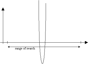
- Sensitivity to expressions which are very fast-changing relative to the requested range, and change back to the initial sign very quickly.†
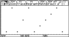
† This situation may look something like this:
The algorithm for the half-step method is simple. Here is a non-mathematical description of it:
Variables: e - the expression
target
- the target
x1
- lower boundary of search range
x2
- upper boundary of search range
tol
- error tolerance within which to accept solution
1. Start at x = x1.
2. Set step size = distance between x1 and x2
3. Store the sign of the value e(x) - target
in initsign.
4. Initialize the variable nosol with true if |
e(x) - target | > tol is true. Othewise
false.
5. While nosol is true do
6. Add step size to x
7. If x > x2 then we
have reached the rightmost boundary x2 and need to get back to x1
8. Reset x to x1
9. Reduce step
size by half refine the step so we could
catch the change of sign
10. End
11. Update nosol with true if |
e(x) - target | > tol is true. Othewise
false.
12. If sign( e(x) - target
) <> initsign and nosol is true then we
have found a change of sign
13. Substract step size from
x take one step back
14. Reduce step size
by half now we would move forward only
half the distance
15. End
16. End
? Hmmm... What was that...? A "simple", "straightforward" method? ; )
Ans
It may seem to be a bit cumbersome, but if you'll take a closer look, you'll
notice that only the
most basic mathematical operations are required: addition, absolute value
and sign. It does not use differentiation, or expressions that include divisions
(may cause problems when denominator approaches zero).
Initial
values are also not used, but only a range, which in most cases is faily easy
to determine (and in any case note the fourth advantage mentioned above).
This method is straightforward in the sense that it requires only elementary
math, and has a logical, easy to follow principle with very little exceptions.
The algorithm in TI-BASIC
Input: e - the expression
var
- the independent variable
target
- the target
x1
- lower boundary of search range
x2
- upper boundary of search range
tol
- error tolerance within which to accept solution
Output: x* - the value of var which brings e to target
within the error tolerance tol
Local Variables: step - holds the current step size
initsign
- holds the first sign of the expression e(x) - target
nosol
- holds true if solution has been found, otherwise false.
val
- holds the value of e(x) - target
1. Local
initsign, nosol, val
2. expr(string(e | var = a)&">e(a)")
turns the expression into a function
of the given variable
3. x1 > x
4. x2 - x1 > step
5. e(x) - target > val we
save the result in a variable, so we won't have to calculate it a second time
6. sign(val) > initsign
7. abs(val) > tol > nosol this
simply puts true or false into nosol
8. While nosol
9. x + step >
x
10. If x > x2 Then
11. x1
> x
12. step
/ 2 > step
13. EndIf
14. e(x) - target
> val
15. abs(val) > tol
> nosol
16. If sign(val) <> initsign
and nosol Then
17. x - step
> step
18. step
/ 2 > step
19. EndIf
20. EndWhile
21. Return x
Clearly, a few crucial aspects are missing from the last algorithm. Namely: a way to stop it through a maximum number of iterations, or when there is no solution in the range, and it tries to catch the change of sign by reducing the step without end. The following is the complete program, plus visual results display and a final graphing of the convergence process.
Input: e - the expression
var
- the independent variable
target
- the target
range
- lower and upper boundary of search range in a list
tol
- error tolerance within which to accept solution
Output: x* - the value of var which brings e to target
within the error tolerance tol
xlist
- a list containing values the values of var through which the algorithm
went.
ilist
- a list containing a sequance of the iterations corresponding to the values
in xlist.
(the
last two output variables are only for our educational purposes)
Local Variables: step - holds the current step size
x
- the current value of var
initsign
- holds the first sign of the expression e(x) - target
nosol
- holds true if solution has been found, otherwise false.
val
- holds the value of e(x) - target
i,
mi - counters for iterations and missed iterations number.
maxi
- holds the maximum number of iterations allowed
maxmi - holds the maximum number of missed iterations allowed
sgn
- this variable will be a sign function, but which includes zero as positive
0. halfstep(e, var,
target, range, tol)
1. Prgm
2. Local initsign, nosol, val, i, mi, maxi, maxmi, sgn, step, x
3. when(x >= 0, 1, -1) -> sgn(x) this
makes a modified sign functions which includes a positive zero
5. 1 -> i
6. 0 -> mi
7. 50 -> maxi
9. 3 -> maxmi
10. expr(string(e | var = xyz)&">e(xyz)")
turns the expression into a function
of the given variable
11. range[1] > x
12. range[2] - range[1] > step
13. e(x) - target > val we
save the result in a variable, so we won't have to calculate it a second time
14. sgn(val) > initsign
15. abs(val) > tol > nosol this
simply puts true or false into nosol
16. {x} -> xlist
17. While nosol and i < maxi and mi < maxmi
18. x + step > x move
forward one step size
19. If x > range[2] Then we
have reached the rightmost boundary of the given range
20. range[1] > x reset
x to leftmost point
21. step / 2 > step refine
step size
22. mi + 1 -> mi update
number of missed iterations
23. EndIf
24. x -> list[i+1] update
x's list
25 e(x) - target > val
26. abs(val) > tol > nosol
27. If sign(val) /= initsign and nosol Then
28. x - step > step move
back one step size
29. step / 2 > step refine
step size
30. EndIf
31. i + 1 -> i update
number of iterations
32. EndWhile
33. ClrIO
34. If i = maxi Then
35. Disp "Max number of iterations"
36. Disp "reached with "&string(var)&"
= "&string(x)
37. ElseIf mi = maxmi Then
38. Disp "Max number of missed iterations"
39. Disp "reached with "&string(var)&"
= "&string(x)
40. Else
41. Disp "Ended with "&string(var)&" =
"&string(x)
42. Disp "Error = "&string( e(x) - target
)
43. Disp "Iterations: "&string(i)
44. EndIf
45. Disp ""
46. Pause "Press [ENTER] ..."
47. If i>1 then
48. seq(j, j, 1, i) -> ilist
49. NewPlot 1, 1, ilist, xlist,,,,4
50. ZoomData
51. Else
52. DispHome
53. EndIf
54. EndPrgm
For your convenience, you can download the program here: TI-89, TI-92+
As shown in line 3, it is very convenient to use when( when a function
operates on a conditional base. If we had written sgn( in full, we
would have written something like this:
sgn(x)
Func
If x >= 0 Then
Return 1
Else
Return -1
EndIf
EndFunc
Obviously, when a single, simple condition is involved, it is much quicker to define the function using when(
Sometimes we need the user to enter an expression and a variable to work
with in that expression, such as in this example, or as used in many functions
on the TIs (for example: d(expression, variable) ).
In the absence of other options, we would have had to evaluate the expression
with respect to variable, when variable has the value of value
in the following way:
expression | variable
= value
For example, the program we've written halfstep( takes an expression e and a variable var. Normally, we would have had to write: e | var = 2 -> b every time we wanted to evaluate e when var is 2, and assign it to b.
There is a better solution. If we could make a function e(var), then
it would be much easier to write e(2), than all the above. The method
is to write, in the general case, something like this:
expr(string(expression
| variable = xyz)&">f(xyz)")
This creates a function f(, which can be used instead of the longer
combination. The variable xyz is just an intermidiate variable, and
the funny name was chosen so as to make sure that no such variable already
exists (that would simply return an error). The variable f can be local,
or global (i.e. it can be declared for use inside the program only, with Local
..., or it can be made a variable that comtinued to exist after the program
has finished).
Here we've simply reused the variable e (line 10), so that it will be local and we wouldn't use memory on another variable (even local variables take memory...)
In line 15 we use a short way to assign true or false to the variable nosol. The long, formal way would have been to write:
If abs(val) >
tol Then
true -> nosol
Else
false -> nosol
EndIf
As before, the short way is shorter, and not much remains to be said.
In accordance with tip 3.10 in Doug Burkett's The TipList, it is faster to append to the list, rather than to use the function augment(. This is implemented here in line 24. Notice that the first value of x is already stored in the list in line 16, and so we begin appending from index 2, and this is the reason for the i + 1. If the list is started from blank, then we begin from index 1, as this little example shows:
{} -> list
For i, 1, 5
i -> list[i]
EndFor
This creates the list {1, 2, 3, 4, 5}.
Note that as error will occur if the program tries to append to an indexs
greater than the last + 1.
The command which defines a plot is called NewPlot, and we use it in line 49. The general syntax is:
NewPlot n, type, xlist, ylist,,,, mark
No, the four commas are not a typo. The reason is that there can appear other options in between, which we ignore here (please consult your manual for a complete description of how to use NewPlot).
n is the plot number
(1 for Plot1, 2 for Plot2, etc.)
type is 1 or 2, for scatter and xyline respectively.
xlist contains the x values
ylist contains the corresponding y values
mark is 1 for box, 2 for cross, 3 for plus, 4 for square and 5 for
dot.
The only catch is this: the lists have to be global variables! In other words,
it wouldn't work to write:
NewPlot
1, 1, {1, 2, 3}, {1, 2, 3},,,, 4
Though the lists are lists, the are not variables,and so this would create
and error.
Think about it this way: with the command NewPlot you are asking to define
a plot using two lists. However, this means that the plot has to be available
later, while a quick look at the plot definition dialog box shows us that
it does not store the lists itself (the values themselves), but only the lists
names.

This is the reason the variable xlist is not a local variable, and likewise ilist isn't, in line 48.
After this command, which only defines the plot, the TI does not automatically switch to the graph screen. We do this manually with the ZoomData command in line 50, which adjusts the window limits to those of the data points.
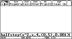
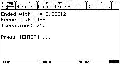
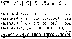
We will use a simple example here: finding when f(x)=x² is 4, with an error tolerance of 0.001.
We first start with a 'good' range: [0 .. 5].
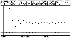
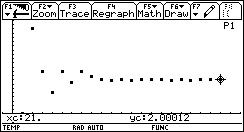
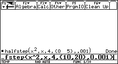
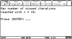
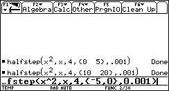
The explanation is obvious: the algorithm couldn't find a sign change between 10 and 20, so it decreases its step size again and again, until the entire range is missed for the 3rd time (this is maxmi).
A negative range [-5 .. 0] will give the other solution:

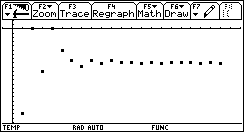
[-100 .. 100]. This is what happens:
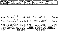

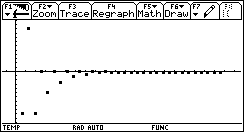
As expected, the algorithm converged to the negative solution (because it is the first, whereas the positive is the second, in terms of the algorithm's progress).
Notice the price for our exaggerated large range of [-100 .. 100]: only 11 more iterations! 50% more iteartions than when we gave the range [-5 .. 0] ! Considering the fact that the range was now 40 times bigger than [-5 .. 0], this is remarkable.
Let's try an even more exagerrated range: [-1000 .. 1000]. How many more iterations will it take this time (the range will be 400 times larger than [-5 .. 0])?
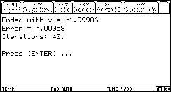
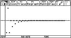
It now took 40 iteartions to converge to a solution! This is twice as much as with [-5 .. 0], when the range is 400 times larger!
Obviously, this method is not the best, when it comes to root finding. We have seen its slowness, even when the range boundaries ware very close to the solution. On the other hand, we have seen it's speed, when the range boundaries are very far from the solution.
This example is long enough already, so we will not discuss other, more delicate cases now. For the educational purposes, I rest my case :)
Congratulations! You have completed this task!
______________________________________________________________________________________
Created by Andrew Cacovean, March 16, 2002